
If you haven’t read Part I and Part II of this series, it’s suggested that you do so. The webinar versions can also be found on our site or on YouTube.
This session will discuss the following:
More with Functions and Formulas
Documenting and Auditing
Using Templates
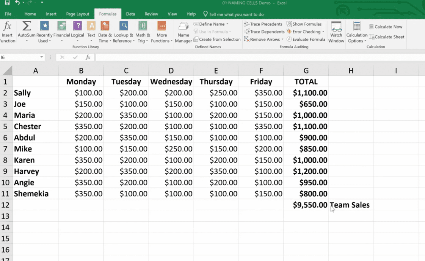
How do you name a cell? You do so by the cell’s coordinates, such as A2 or B3, etc. When you write formulas using Excel’s coordinates and ranges you are “speaking” Excel’s language. However, this can be cumbersome. For example, here G12 is significant because it refers to our Team Sales.
You can teach Excel to speak your language by naming the G12 cell Team Sales. This will have more meaning to you and your teammates. The benefits of naming cells in this fashion are that they are easier to remember, reduce the likelihood of errors, and use absolute references (by default).
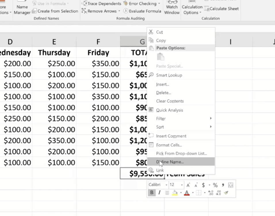
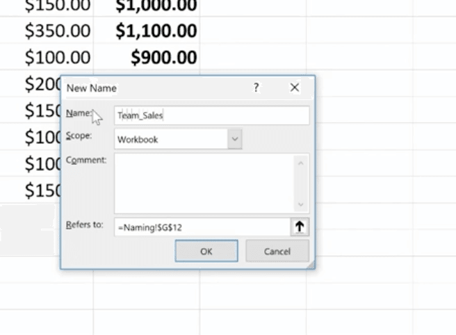
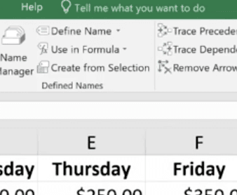
To name our G12 cell Team Sales, right-click on the cell, choose Define Name, and type “Team Sales” into the dialog box. You can also add any comments you want here. Then click Ok.
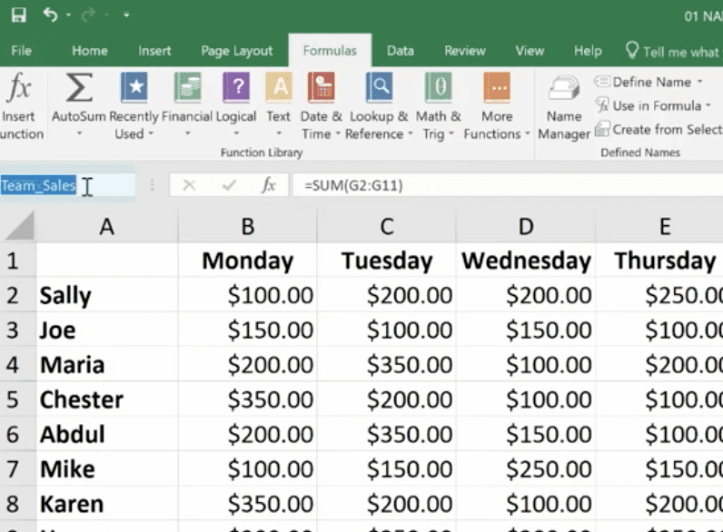
Another way to do this is to click on the G12 cell and go up to the Name Box next to the Formula Bar, then type your name there.
And, there’s a third option at the top of the page called “Define Cells” that you can use.
Notice that there’s an underscore between Team and Sales (Team_Sales). There are some rules around naming cells:
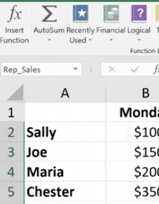
Highlight an entire range of cells and name your range (we’re doing this in the upper left-hand corner).
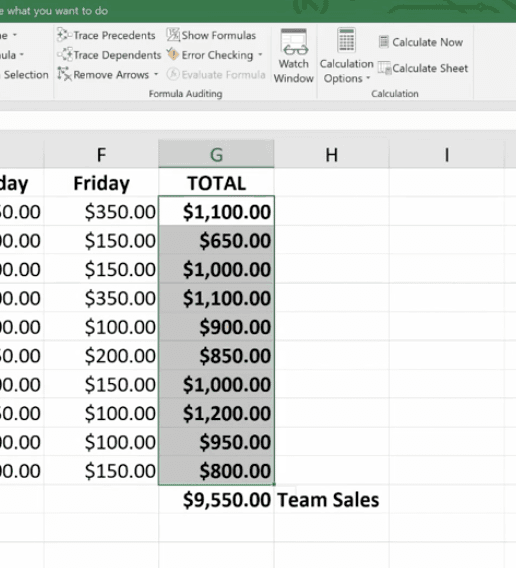
Then you can easily use the name to produce the sum you need:
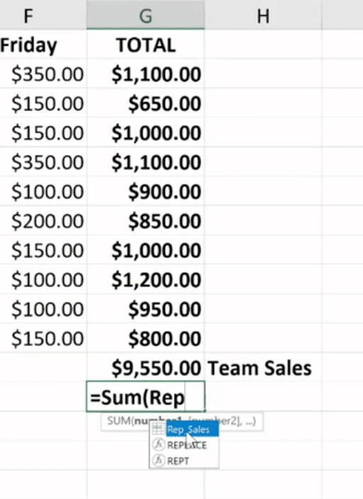
You won’t have to go back and forth from spreadsheet to spreadsheet clicking on specific cells to calculate your formula. You simply key in the name of the cell range you want to add. Just be sure to remember the names as you build your spreadsheets over time.
If you ever make a mistake or want to change names, you can go to Name Manager to do this.
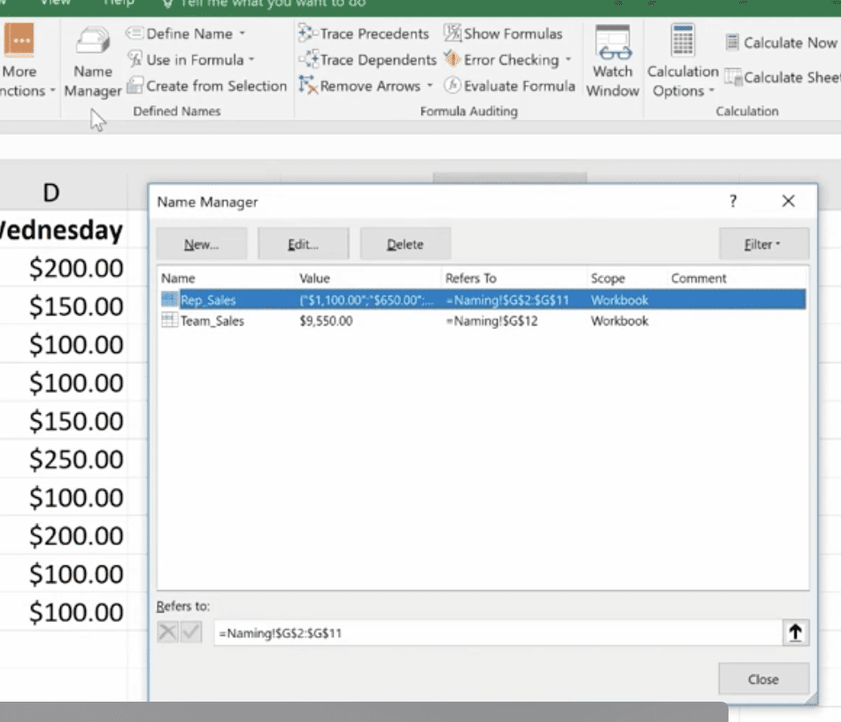
Remember that if you move the cells, the name goes with it.
The three statistical functions are:
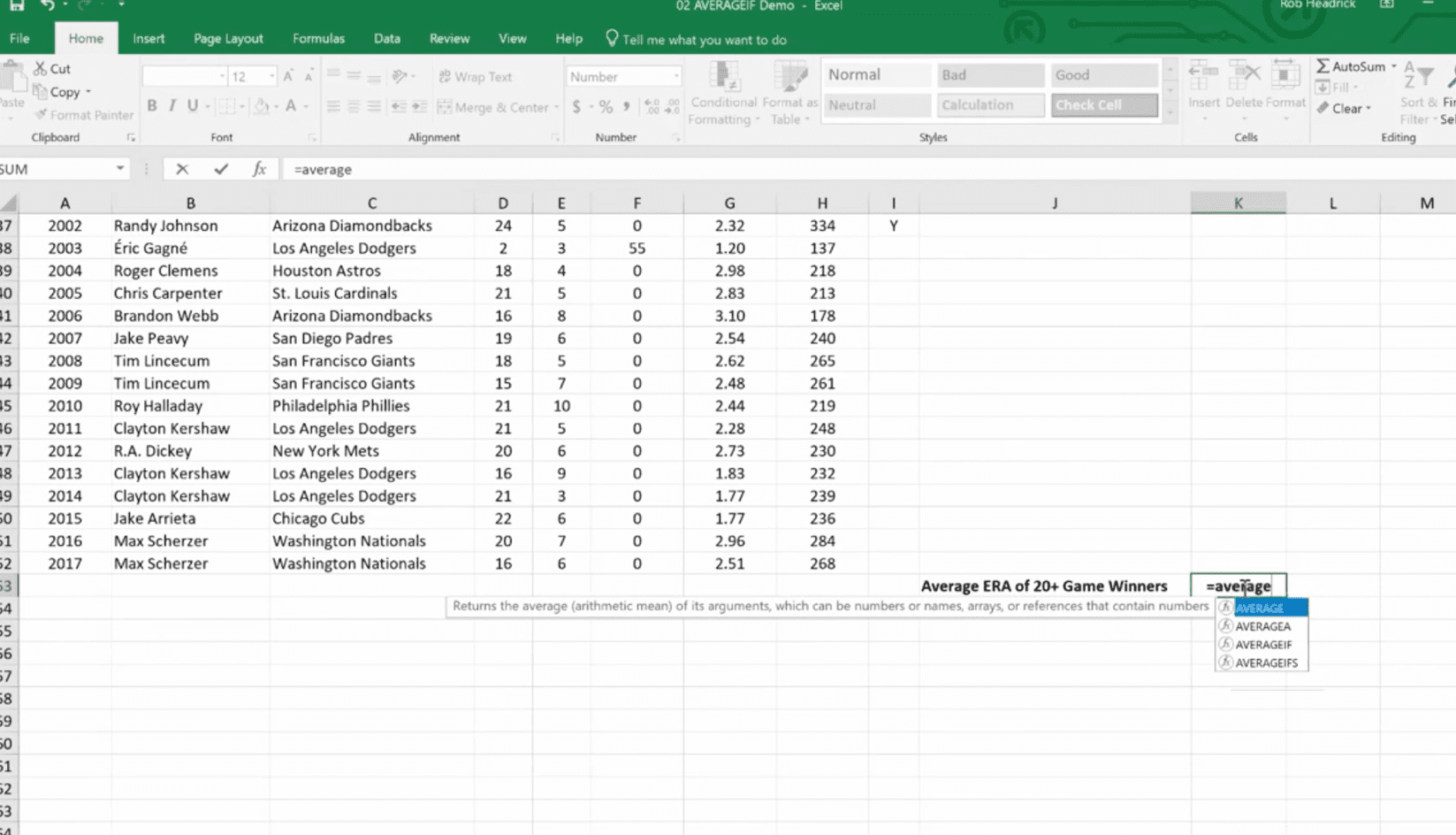
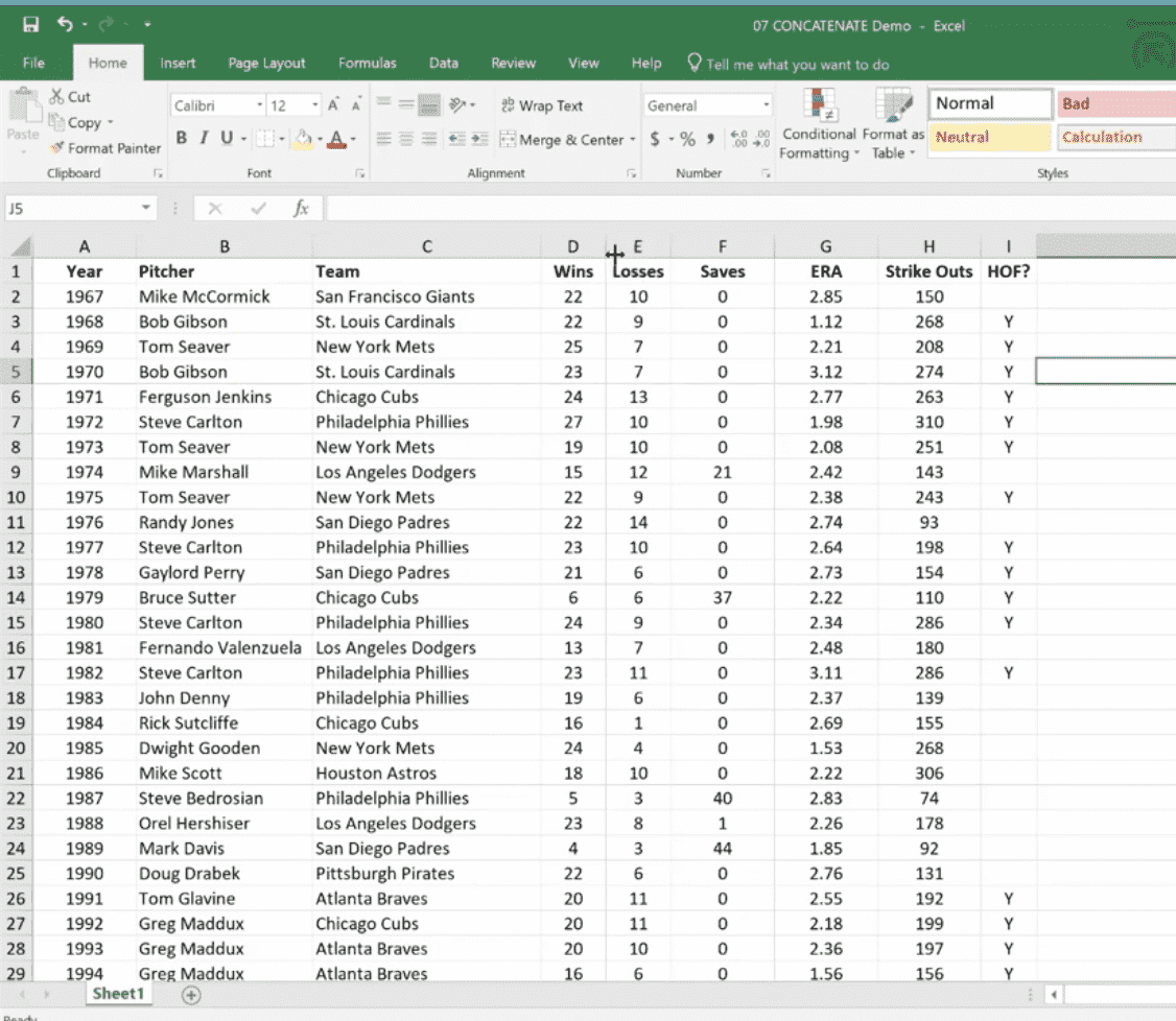
The Average If can be used to figure out the average of a range based on certain criteria. Here we’re going calculate the Average If of the ERA of 20+ Game Winners from the spreadsheet we developed in our last session.
We’ve already named some of our cell ranges (wins, era). And we want to know the average greater than 19.
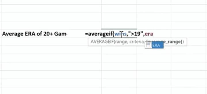
Hit Enter and you have the average.
You can use this feature across a wide variety of scenarios. For example, if you wanted to know the average sales of orders above a certain quantity – or units sold by a particular region, or the average profit by a distinct quarter.
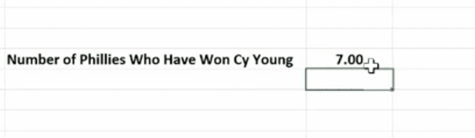
Count If is used for finding answers to questions like, “How many orders did client x place?” “How many sales reps had sales of $1,000 or more this week?” or “How many times have the pitchers of the Philadelphia Phillies won the Cy Young Award?”
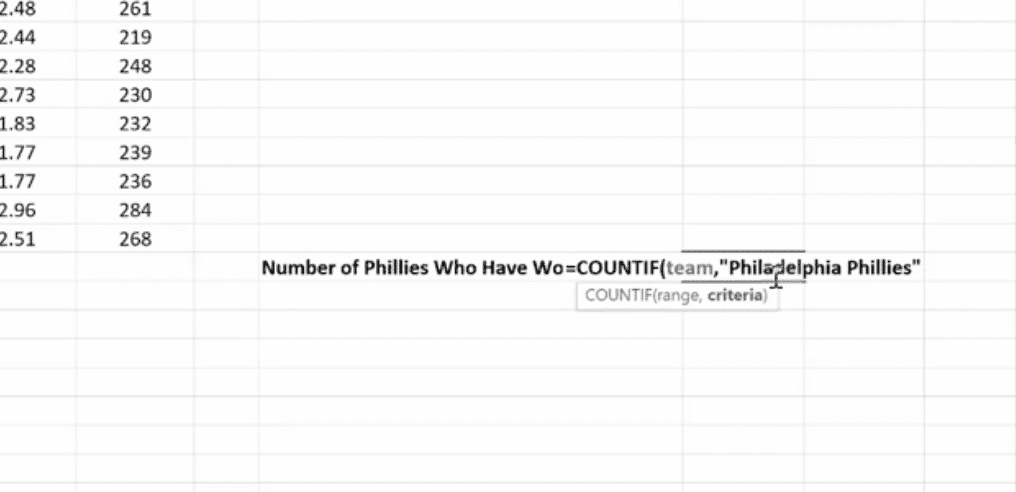
As you can imagine, it’s essential that you type in the text exactly the way you named that particular cell.
Hit Enter and you get your answer
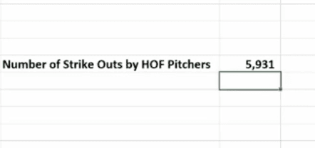
Now we’re going to use the Sum If function to calculate the number of strikeouts by the pitchers on this list who are in the Baseball Hall of Fame.
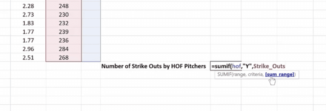
Sum If is a good way to perform a number of real-world statistical analyses. For example, total commissions on sales above a certain price, or total bonuses due to reps who met a target goal, or total earnings in a particular quarter year-over-year.
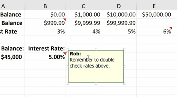
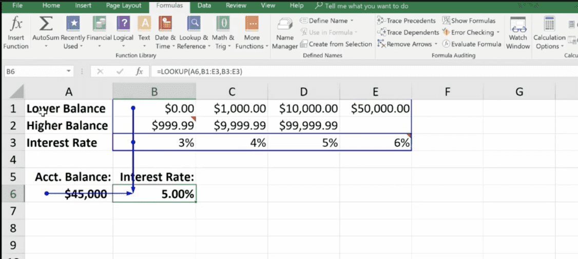
These are designed to ease the finding and referencing of data, especially in large tables. Here, cells A1 and E3 relate to a variable interest rate that is paid on a bank account. For balances under $1,000, the interest rate is 3% – between $1,000 and $10,000, the interest rate is 4%, etc.
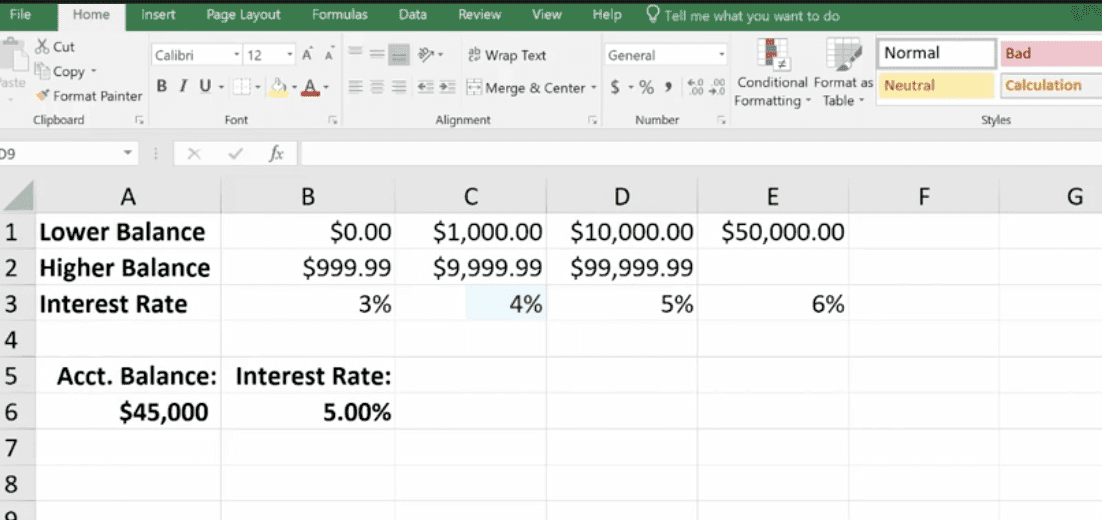
Cell A6 shows the balance of a specific account. The Lookup Function is used in B6. It looks up the interest rate and applies it to the account balance of $45,000. This is what the formula looks like in the bar at the top:
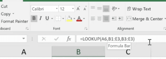
The vector form of the Excel Lookup Function can be used with any two arrays of data that have one-to-one matching values. For example, two columns of data, two rows of data, or even a column and a row would work, as long as the Lookup Vector is ordered (alphabetically or numerically), and the two data sets are the same length.
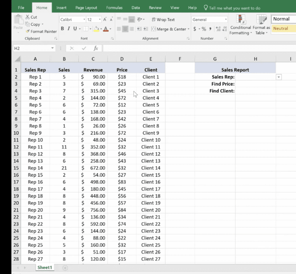
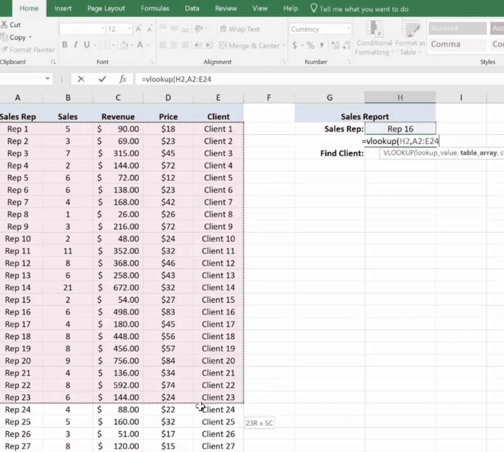
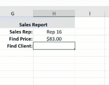
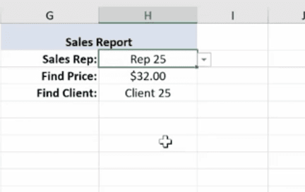
V Lookup and H Lookup are used to pull information into reports. We’re going to use Report Setup. Here, we have a worksheet that references salespeople, sales data, pricing, revenue, and the clients that they sold to. You’ll see on the top right where we set up a report with names referencing sales data.
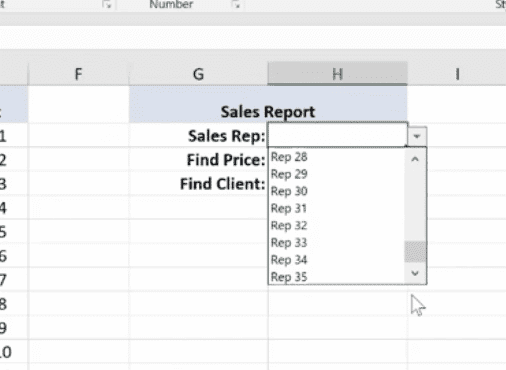
You can access the sales reps in the drop-down menu. Pick a rep and use the V Lookup Function to find the price.
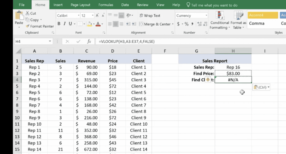
To Find Price, key in =vlookup and the corresponding cell number for Rep 16, plus the table array which is the entire table not including the header at the top.
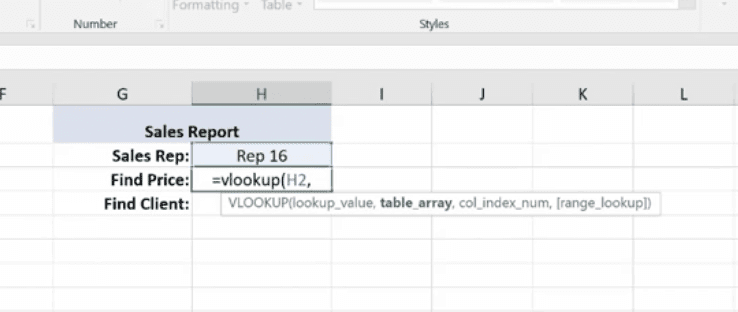
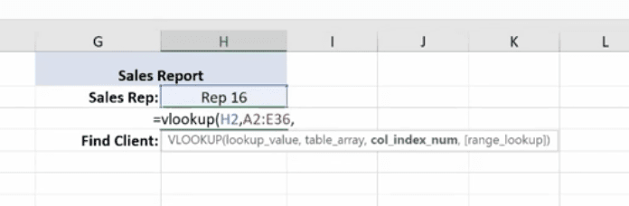
Then you need the column index number. This is the number of columns to the right of your lookup value column, which is column A. It’s the 4th column from column A (Price).
Enter 4,
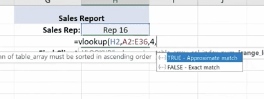
For range lookup we’re using true or false. We are entering false here.
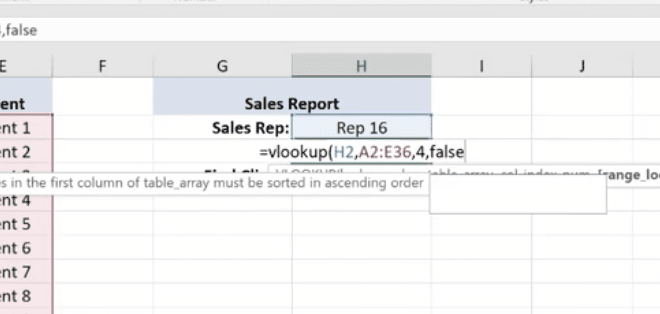
Hit Enter and this is what you have for your Find Price value.
Now we’ll do a similar V Lookup for the Client. Copy and Paste:
Make the necessary changes in your formula:
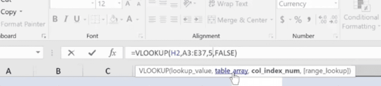
Client 16 goes with Rep 16. 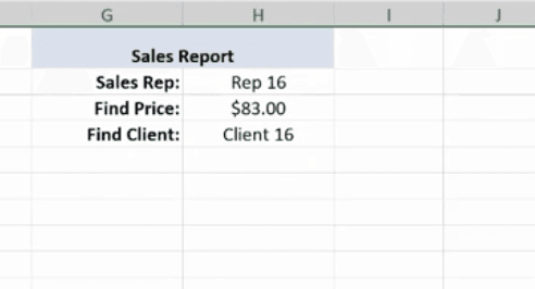
Note: If you change the Sales Rep, all the corresponding values will change.
If you have a lot of data and long tables, V Lookup helps you find information easily. The V stands for Vertical (or by column), because columns are vertical. H Lookup is for Horizontal-like column headers.
Text Functions contain some very powerful tools to adjust, rearrange and even combine data. These functions are used for worksheets that contain information and function as a database such as mailing lists, product catalogs, or even Cy Young Award Winners.
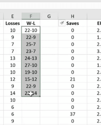
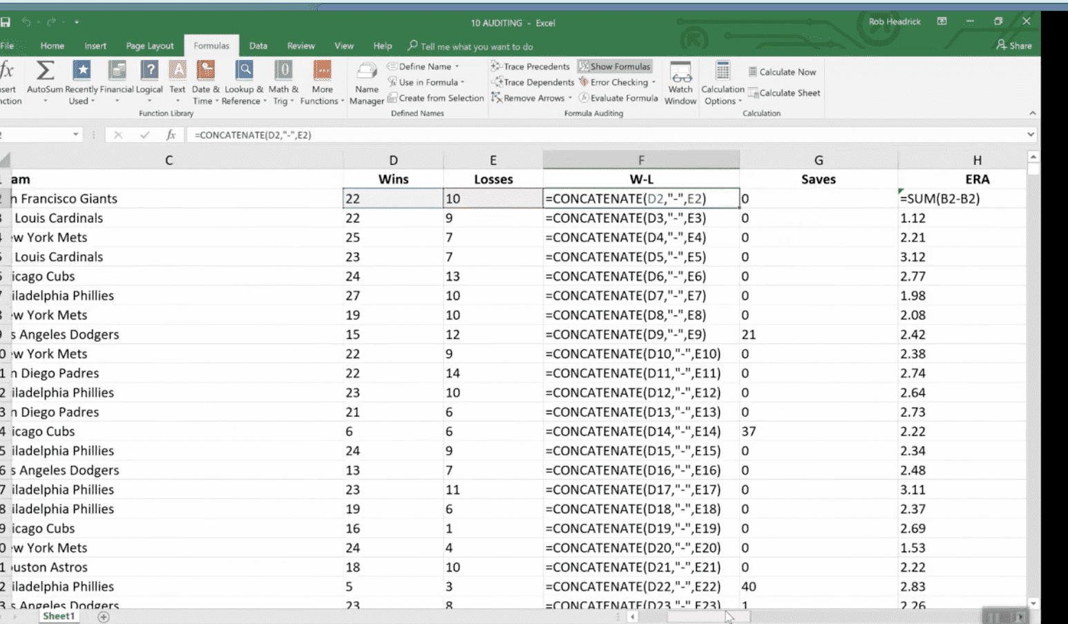
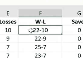
The first text function we’ll show you is concatenate. It links things together in a chain or series. Here, we have our Cy Young list. But we no longer need to see our Wins and Losses in a separate column.
To do this easily rather than manually, create a new column where your data will reside.
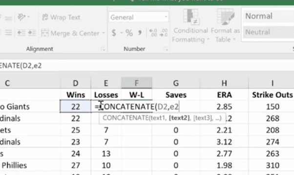
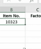
Hit Enter
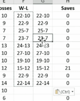
Now, just go in and hide the Wins and Losses columns. Don’t delete them or your new column will have a reference error.
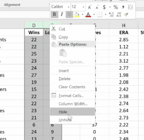
If you do want to delete the Wins and Losses columns, you must first make a new column. Copy the W-L numbers and Paste Value in the new column. This way you’ve moved from a formula to the new information. If you delete your source information without taking this step you’ll be left with nothing.
Combine as many columns as you need with the concatenate function to make the data appear as you need it to.
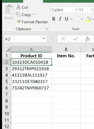
These are used to tell Excel that you only want part of a text string in a particular cell. Here, we have a product list and product IDs that tell us the date of manufacturer, the item number, and the factory where it was made. We’re going to pull the data out so we can put it in columns to use in different ways.
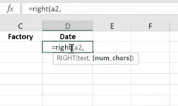
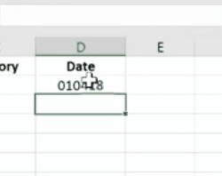
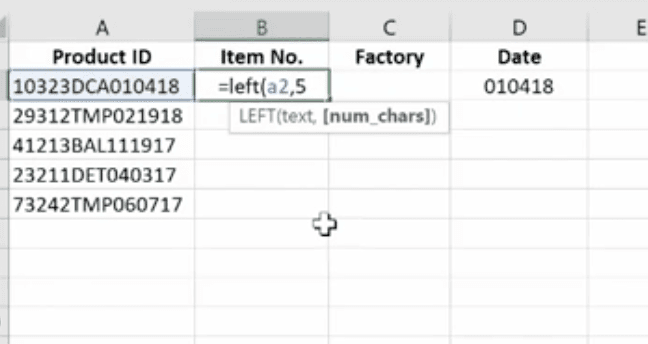
We use the Mid Function here.
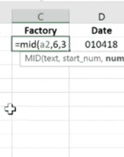
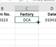
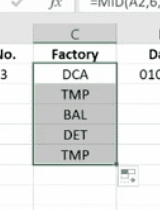
This works because each of the product IDs are the same length. If they were different lengths you’d have to do something more creative.
You want to make your Excel files easy to understand for both yourself and others who need to use them – and this includes auditors. An organized worksheet results in clear error-free data and functions.
The purpose of commenting is to provide notes to yourself or especially to others. Comments can include reminders, explanations or suggestions.
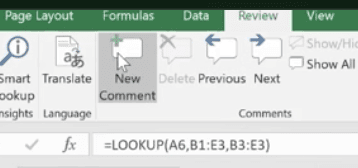
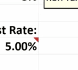
You’ll find the New Comment button at the top under the Review Menu. Simply click the cell where you want the comment to go and click New Comment. Then type your comment and click outside the box to close it. The comment will disappear but it’s still there. Anywhere you see a red flag, there’s a comment.
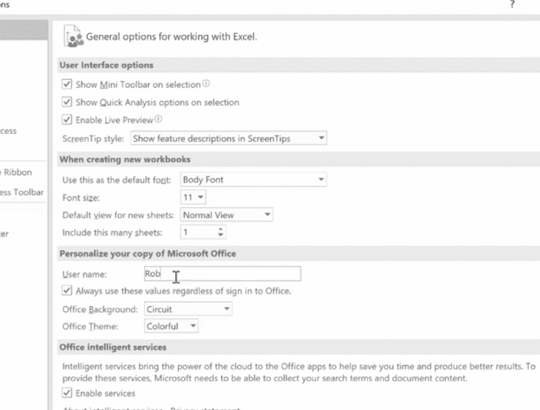
If your name doesn’t appear in the comment, go to File>Options>General and personalize your copy of Excel (in this case Microsoft Office) under the User Name. You won’t need to go back and change each comment; Excel will do this for you.
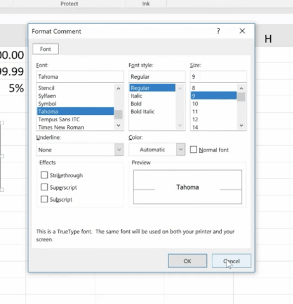
To format a comment, click inside the comment box and a drop down will come up where you can format the text.
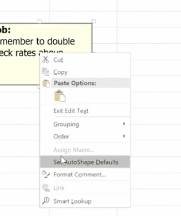
You can change the color of the box and lines around the box. Some managers have different colors for members of their teams.
If you change the default color, it will change that for all your Microsoft products.
To delete a comment, go to the cell that hosts it, then go up and hit delete.
If you have a lot of comments, grab the handle on the box and resize it.
What we really mean is formula auditing. This is an advanced way to check your work.
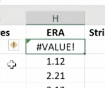
The yellow diamond on the left of this cell indicates that there’s an error.
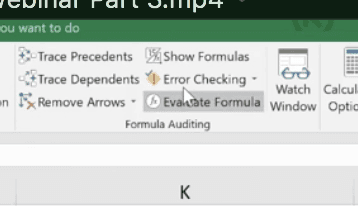
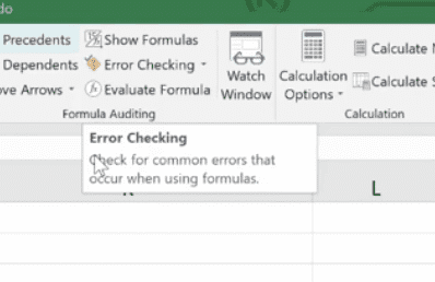
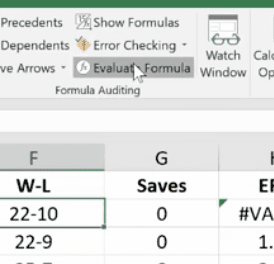
Or to find any errors, go to Formula Auditing in the top menu.
You have a number of helpful tools here. Trace Precedents shows where the formula looks for information. Click the formula you want and click Trace Precedents. It will display where your data came from.

Here’s a more complex formula and trace auditing:
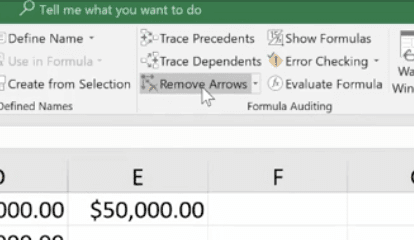
To hide the arrows, click “Remove Arrows.”
This expands all of your columns and shows all of them in a bigger way. You can go in and check your formulas on the fly very easily. Click Show Formulas again and the worksheet goes back to the way it was before.
This feature lets you check all formulas at once.
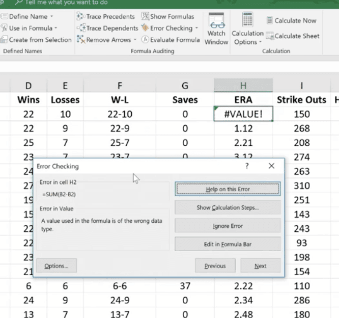
This makes it easy to find errors and correct them.
This feature allows you to check a formula step-by-step. It shows the results of each individual part. It’s another great way to de-bug a formula that isn’t working for you. Click the formula you want to evaluate. Click Evaluate Formula and you’ll get a dialog box.
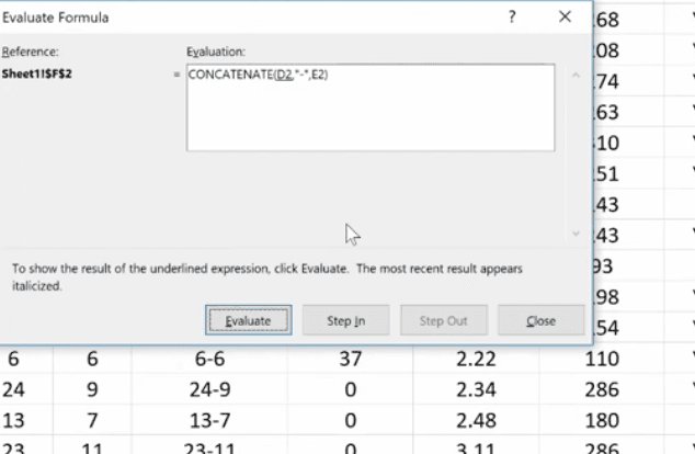
Click Evaluate and it will change the formula to the actual value that you can review. Each time you click Evaluate, it will take you through the steps of how you got to the final formula. You can trace your way through to see if you made any errors.
With protection you can lock in your changes in individual cells, spreadsheets, and entire workbooks. You can also protect comments from being moved or edited.
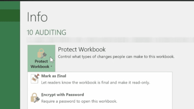
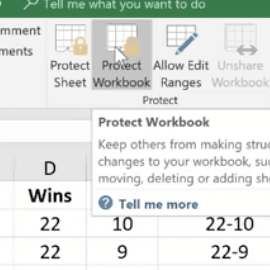
This is how to protect an entire workbook. It’s the highest level of protection.
You’ll want to do this if your workbook contains confidential information like:
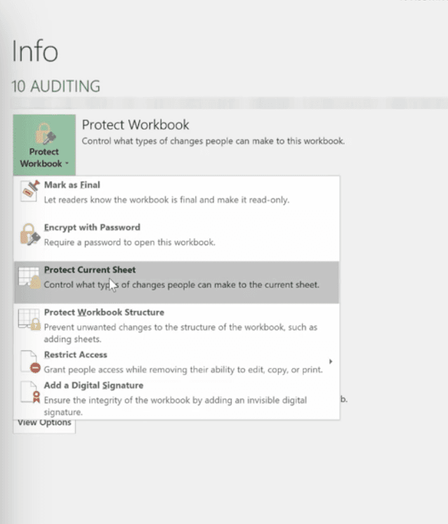
Click File>Info>Protect Workbook>Encrypt with Password.
Enter your password and be sure to make note of it because it can’t be recovered if you lose it. You can use password management software to keep track of your passwords.
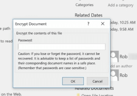
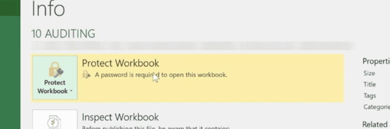
Once complete, click OK and your Protect Workbook function turns yellow indicating that you’ve protected your workbook.
To take off protection, retrace your steps.
You can also protect a current sheet you’re working on. It will take you back to your worksheet where you’ll be presented with a variety of options.
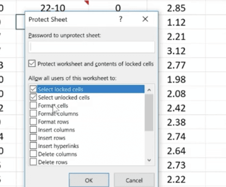
You can also protect cells and comments from this option.
In the same way you protected the worksheet, you can protect your workbook.
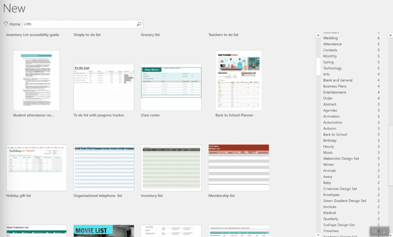
To see the variety of templates you can use in Excel, click File>New and you’ll be presented with a collection of 25 templates you can choose from.

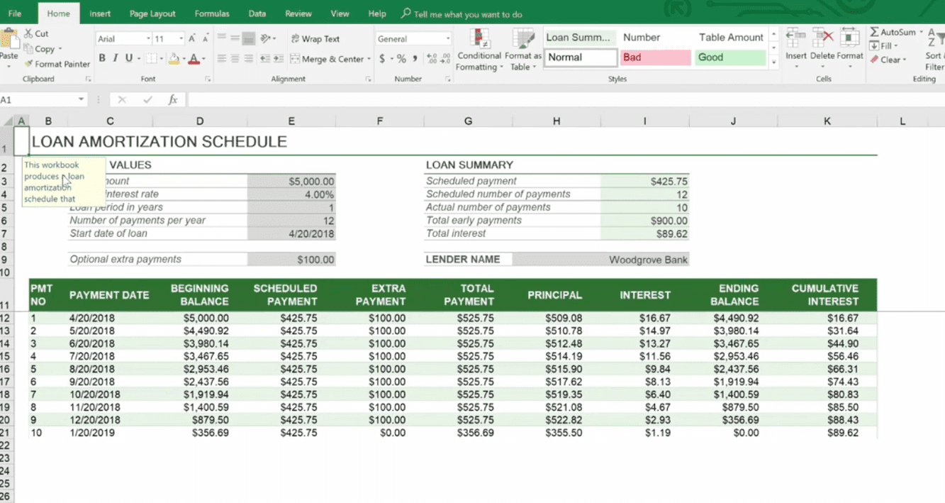
For example, there’s a great Loan Amortization Schedule you can use. Formulas are built in for you. All you need to do is change the numbers.
You can also go online while inside Excel to find more. You don’t want to download templates from outside Excel because they may contain macros that are contaminated with viruses.
On the right side of the page, you have a huge selection to choose from.
It even provides employee time sheets you can use that can save you so much time trying to figure out formulas. 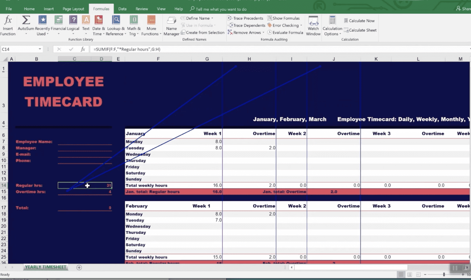
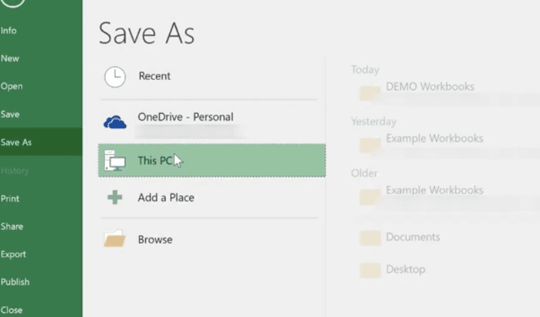
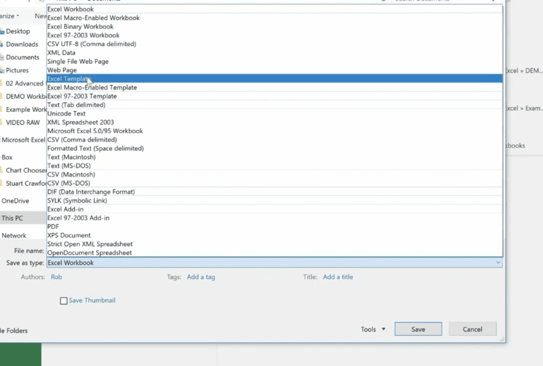
Go to File>Info>Save As and save the template to your location, then save as an Excel Template.
Before you save as a template you want to:
Congratulations! Now you’re an Excel Pro! This completes our Excel Like a Pro Series. If you have any questions or need assistance, feel free to contact our Excel 2016 experts.
Call our business managed IT services department directly at (404) 777-0147 or simply fill out this form and we will get in touch with you to set up a getting-to-know-you introductory phone call.
Fill in our quick form
We'll schedule an introductory phone call
We'll take the time to listen and plan the next steps
11285 Elkins Rd Suite E1, Roswell, GA 30076
Hours: Monday - Friday
8:00 am - 5:00 pm
Hours: Monday - Friday
8:00 am - 5:00 pm

If you want our team at Centerpoint IT to help you with all or any part of your business IT, cybersecurity, or telephone services, just book a call.

We are turning 15 and want to celebrate this milestone with you because without you this would not have been possible. Throughout this year look for special promotions on services and tools aimed at Making IT Simple for You so you can focus on your business.
We are turning 15 and want to celebrate this milestone with you because without you this would not have been possible. Throughout this year look for special promotions on services and tools aimed at Making IT Simple for You so you can focus on your business.